Glossary and acronyms with LaTeX

My template to create glossaries in LaTeX with a description and an associated acronym.  I substitute every term "EEE" by the new glossary term and the term "Expanded" by the expanded version (e.g. EEE -> NYC, Expanded -> New York City).

%%% define the acronym and use the %see= option
\newglossaryentry{EEE}{
  type=\acronymtype,
  name={EEE\glsadd{EEEg}},
  description={Expanded},
  descriptionplural={\glsentrydesc{EEE}s},
  first={\glsentrydesc{EEE} (EEE)\glsadd{EEEg}},
  firstplural={\glsentrydescplural{EEE} (\glsentryplural{EEE})\glsadd{EEEg}},
  %see=[Glossary:]{EEEg}
}

\newglossaryentry{EEEg}{
  name={EEE},
  description={TODO: description}
}

Be careful with the plural of the terms, as in this template it only adds an 's' at the end of the description and acronym, in special cases just modify the fields accordingly.

I store all the glossary terms in a file named glossary.tex in a separated folder 00_frontmatter
You need to load the package glossaries at the beginning of the file. I added some options for the table of contents and something else.

\usepackage[toc,seeautonumberlist,acronym]{glossaries}

 
Then, I add this lines in the preamble of the file (before the \begin{document})

%% GLOSSARY
\makeglossaries
\loadglsentries[main]{00_frontmatter/glossary}

Inside the document where I want to print the acronyms:

\printglossary[type=\acronymtype]

 Finally, at the end of the document I print the glossary with:

\printglossary[type=main]

LaTeX apalike citation style

If you tried the apalike citation format you realized that LaTeX is not able to break the citations into two lines. In this case, LaTex just extends the citation from the margins (expecting that you print in the margins of your publication).

(Image from the original source linked below)

This problem can be solved with the package Natbib created by Patrick Daly. Natbib has additional options but in my case -- in order to simplify thing -- I just loaded the package with the option of square brackets []:

\usepackage[square]{natbib}

And changed all the \cite commands by \citep (see other formats in the wikibooks). Instead of changing the hundreds of citations that I wrote in my thesis, I opted to rename the cite command to citep:

\renewcommand{\cite}{\citep}

The bibliography style should remain unchanged:

\bibliographystyle{apalike}

source: http://tex.stackexchange.com/questions/437/line-breaking-or-hyphenation-of-references-in-apalike/447#447

Remove orphan packages in Debian

deborphan is a program that finds orphan packages and just lists them. It has other options but I am not explaining them here.


In Debian it can be installed just with:

sudo aptitude install deborphan

or

sudo apt-get install deborphan

Then, just run the program to print the list of orphan packages. It does not need root privileges as it only prints out the name of the packages.

deborphane

 Then it is up to you if you want to remove everything or just some of the packages. I am not completly sure if it is safe to remove all of them, read more in the original source.

If you want to remove one of them just use your package manager to remove them as usual:

sudo aptitude remove 'the_name_of_the_package'

Or use "purge" instead of remove to clean completly the package with all its configuration files.

source: https://www.debian-administration.org/article/134/Removing_unnecessary_packages_with_deborphan

Very Deep CNN (19conv) first convolution filters 3D visualization

These are the filters of the first convolution layer of the very deep Convolutional Neural Network from Karen Simonyan and Andrew Zisserman available in the webpage www.robots.ox.ac.uk/~vgg/research/very_deep/ The authors have available an arXiv version of a paper in http://arxiv.org/abs/1409.1556

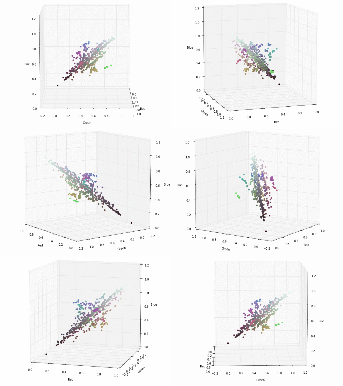
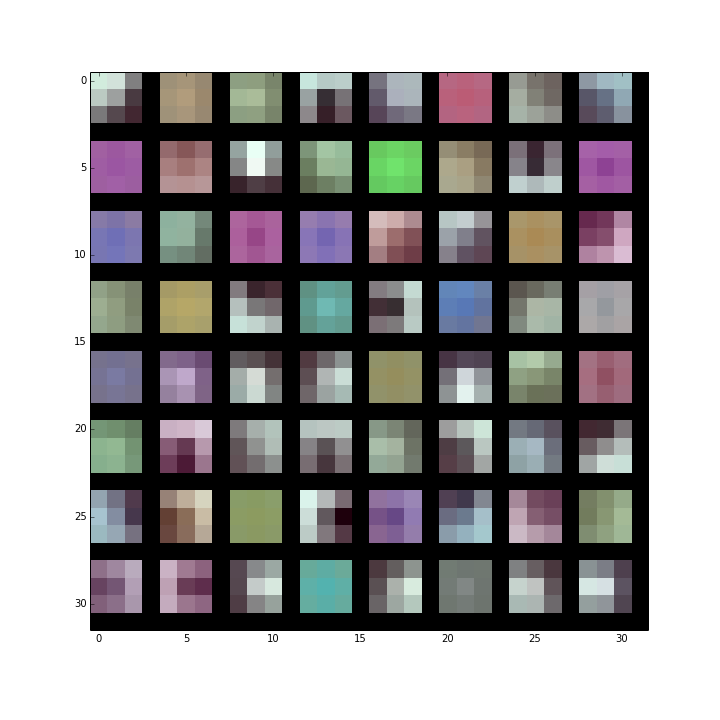
They got the 1st position for the localization task and the 2nd position in the classification task in ImageNet Challenge 2014. In order to get these results they evaluated different architectures with an increasing depth. This is the projection of the first convolutional layer filters in the RGB colorspace. Click on the images to see a 3D representation of the filters components.

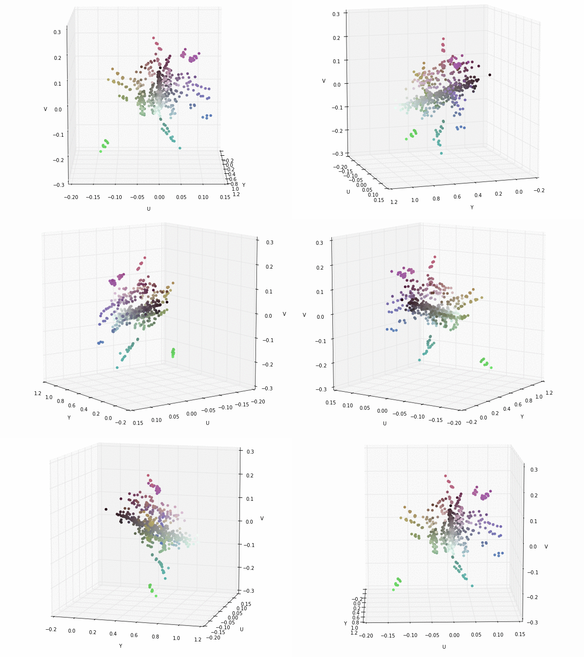
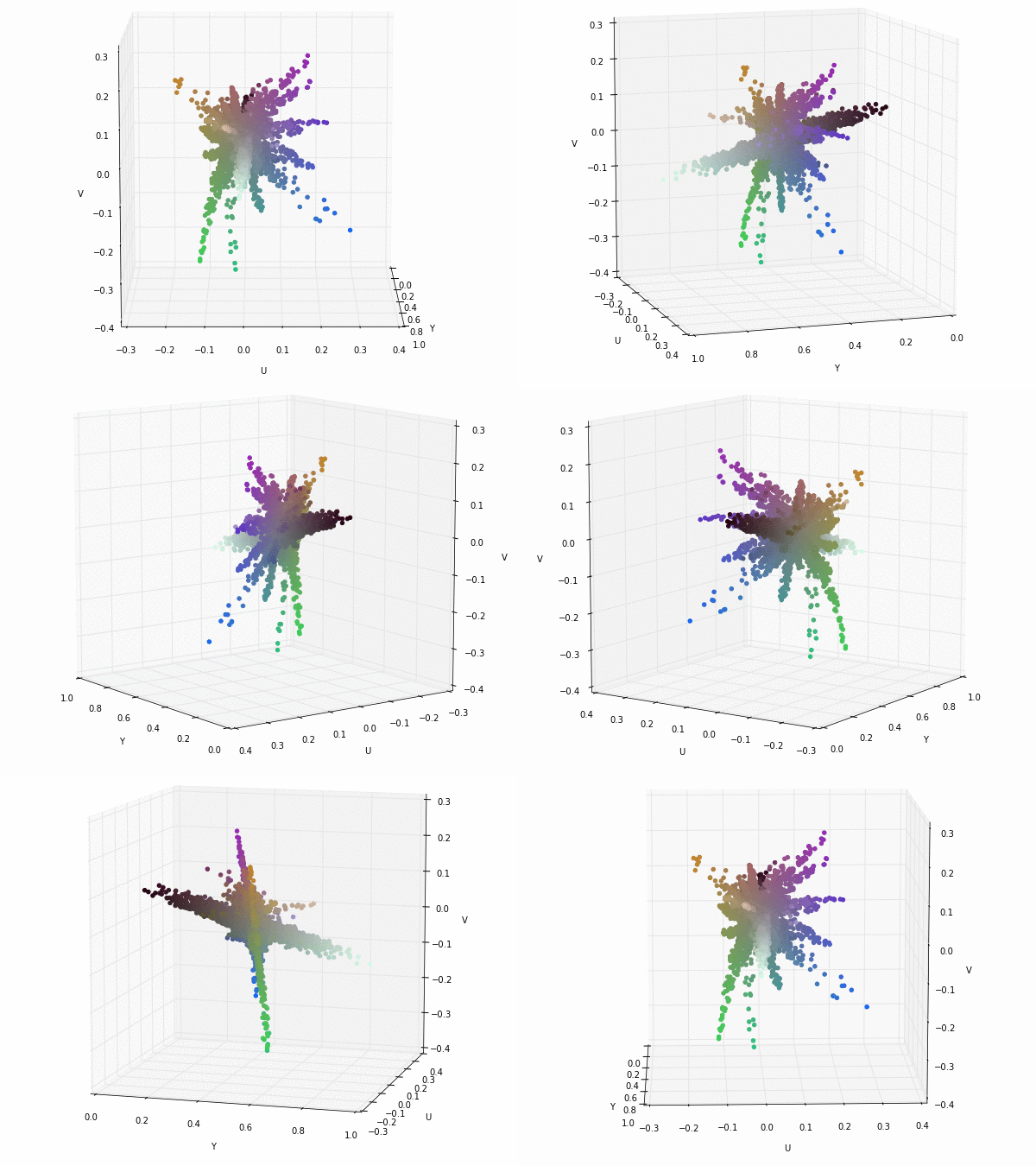
As in the Alexnet example we can do a linear transformation of the original RGB channels and visualize the same colors in the YUV colorspace. In this case the distribution of the points is not that clean and it seems that the distribution of the colours is more spread. This could be because the number of weights is very reduced 64x3x3x3 + 64 = 1792, compared to Alexnet 96x3x11x11 +96 = 34944.

If you find these interesting you can take a look at the results in my Master Thesis: webpage or the pdf and do not hesitate to ask me any question.

Alexnet first convolution filters 3D visualization

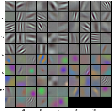
This are the filters of the first convolution layer of Alexnet network. If we look at them, they seem to be interested in luminance patterns (black-gray-white filters) and chrominance patterns (only the colour part without the black-gray-white component). This means that at the beginning the filters are specialized on this two typical situations and after that in the next convolution layer they could be appropriately merged.

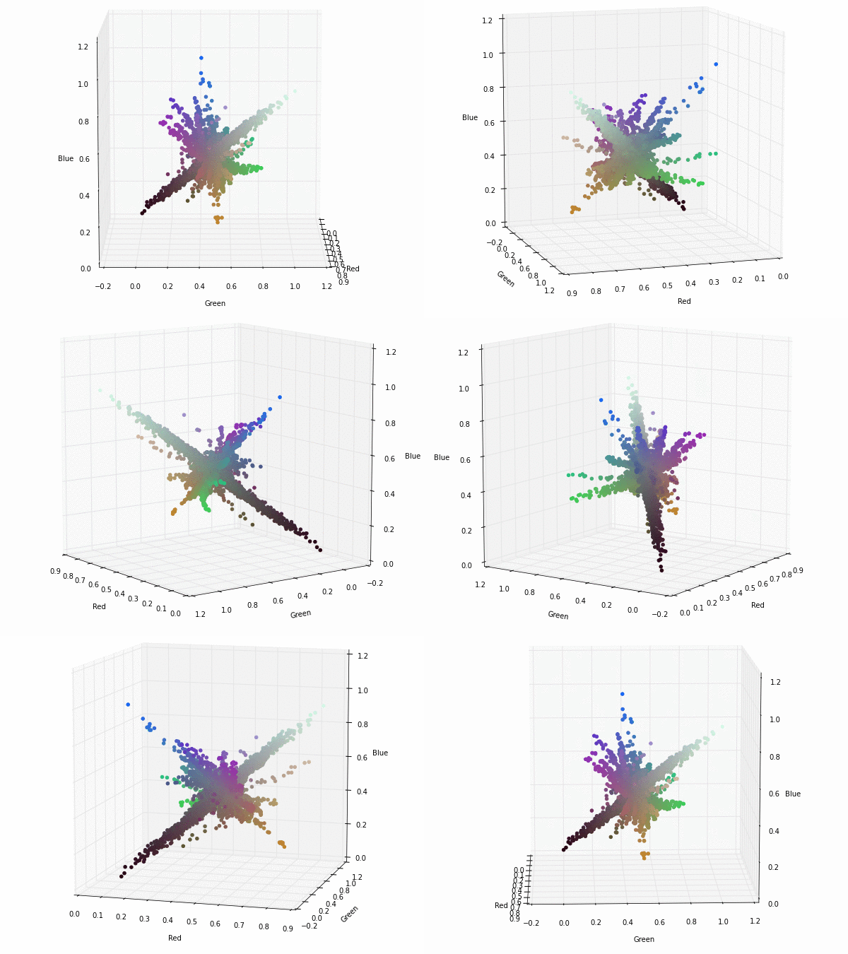
To illustrate that, this is the projection of each pixel of the filters (they are really weight vectors with three components red-green-blue). Click on the images to see a 3D representation of the filters components.

If we apply a transformation to YUV colorspace; also known as YCbCr for digital images. We can see that the Y component (luminance) nearly gets their own axis while UV components (chrominance) are strongly correlated but slightly uncorrelated with the Y component. This means that they could be separated without any problem when training a CNN.

If you find these interesting you can take a look at the results in my Master Thesis: webpage or the pdf and do not hesitate to ask me any question.

Alexnet Graphviz visualization

Visualization of Alexnet using Graphviz. The example is a PNG as Blogger does not accept vectorial images like SVG or PDF. However, with the code below it is possible to generate a PDF calling the program "dot" with the next command:

dot -Tpdf alexnet.gv -o alexnet.pdf
# or an SVG
dot -Tsvg alexnet.gv -o alexnet.svg

alexnet.gv

// ================================================= //
// Author: Miquel Perello Nieto                      //
// Web:    www.perellonieto.com                      //
// Email:  miquel.perellonieto at aalto dot fi       //
// ================================================= //
//
// This is an example to create Alexnet Convolutional Neural Network
// using the opensource tool Graphviz.
//
// Tested with version:
//
//      2.36.0 (20140111.2315)
//
// To generate the graph as a PDF just run:
//
//      dot -Tpdf alexnet.gv -o alexnet.pdf
//
// One think to have in mind is that the order of the nodes definition modifies
// nodes position.

digraph Alexnet {
    // ================================== //
    //  GRAPH OPTIONS                     //
    // ================================== //

    // From Top to Bottom
    rankdir=TB;

    // Tittle possition: top
    labelloc="t";
    // Tittle
    label="Alexnet";

    // ================================== //
    //  NODE SHAPES                       //
    // ================================== //
    //
    // There is a shape and color description for each node
    // of the graph.
    //
    // It can be specified individually per node:
    //      first_node [shape=circle, color=blue];
    //
    // Or for a group of nodes if specified previously:
    //      node [shape=circle, color=blue];
    //      first_node;
    //      second_node;
    //

    // Data node
    // =========

    data [shape=box3d, color=black];

    // Label node
    // =========

    label [shape=tab, color=black];

    // Loss function node
    // ==================

    loss [shape=component, color=black];

    // Convolution nodes
    // =================
    //
    // All convolutions are a blue inverted trapezoid
    //

    node [shape=invtrapezium, fillcolor=lightblue, style=filled];
    conv1;
    conv3;
    // Splitted layer 2
    // ================
    //
    //  Layers with separated convolutions need to be in subgraphs
    //  This is because we want arrows from individual nodes but
    //  we want to consider all of them as a unique layer.
    //

    subgraph layer2 {
        // Convolution nodes
        //
        node [shape=invtrapezium, fillcolor=lightblue, style=filled];
        conv2_1;
        conv2_2;
        node [shape=Msquare, fillcolor=darkolivegreen2, style=filled];
        relu2_1;
        relu2_2;
    }

    // Splitted layer 4
    // ================
    //

    subgraph layer4 {
        // Convolution nodes
        //
        node [shape=invtrapezium, fillcolor=lightblue, style=filled];
        conv4_1;
        conv4_2;
        node [shape=Msquare, fillcolor=darkolivegreen2, style=filled];
        relu4_1;
        relu4_2;
    }

    // Splitted layer 5
    // ================
    //

    subgraph layer5 {
        // Convolution nodes
        //
        node [shape=invtrapezium, fillcolor=lightblue, style=filled];
        conv5_1;
        conv5_2;
        // Rectified Linear Unit nodes
        //
        node [shape=Msquare, fillcolor=darkolivegreen2, style=filled];
        relu5_1;
        relu5_2;
    }

    // Rectified Linear Unit nodes
    // ============================
    //
    // RELU nodes are green squares
    //

    node [shape=Msquare, fillcolor=darkolivegreen2, style=filled];
    relu1;
    relu3;
    relu6;
    relu7;

    // Pooling nodes
    // =============
    //
    // All pooling nodes are orange inverted triangles
    //

    node [shape=invtriangle, fillcolor=orange, style=filled];
    pool1;
    pool2;
    pool5;

    // Normalization nodes
    // ===================
    //
    // All normalization nodes are gray circles inside a bigger circle
    // (it reminds me a 3 dimmensional Gaussian looked from top)
    //

    node [shape=doublecircle, fillcolor=grey, style=filled];
    norm1;
    norm2;

    // Fully connected layers
    // ======================
    //
    // All fully connected layers are salmon circles
    //

    node [shape=circle, fillcolor=salmon, style=filled];
    fc6;
    fc7;
    fc8;

    // Drop Out nodes
    // ==============
    //
    // All DropOut nodes are purple octagons
    //

    node [shape=tripleoctagon, fillcolor=plum2, style=filled];
    drop6;
    drop7;

    // ================================== //
    //  ARROWS                            //
    // ================================== //
    //
    // There is a color and possible a label for each
    // arrow in the graph.
    // Also, some nodes has connections going in and
    // going out.
    //
    // The color can be specified individually per arrow:
    // first_node -> second_node [color=blue, style=bold,label="one to two"];
    //
    // Or for a group of nodes if specified previously:
    //  edge [color=blue];
    //  first_node -> second_node;
    //  second_node -> first_node;
    //  second_node -> third_node;
    //

    //
    // LAYER 1
    //

    data -> conv1 [color=lightblue, style=bold,label="out = 96, kernel = 11, stride = 4"];

    edge [color=darkolivegreen2];
    conv1 -> relu1;
    relu1 -> conv1;

    conv1 -> norm1 [color=grey, style=bold,label="local_size = 5, alpha = 0.0001, beta = 0.75"];
    norm1 -> pool1 [color=orange, style=bold,label="pool = MAX, kernel = 3, stride = 2"];

    pool1 -> conv2_1 [color=lightblue, style=bold,label="out = 256, kernel = 5, pad = 2"];
    pool1 -> conv2_2 [color=lightblue, style=bold];

    //
    // LAYER 2
    //

    edge [color=darkolivegreen2];
    conv2_1 -> relu2_1;
    conv2_2 -> relu2_2;
    relu2_1 -> conv2_1;
    relu2_2 -> conv2_2;

    conv2_1 -> norm2 [color=grey, style=bold,label="local_size = 5, alpha = 0.0001, beta = 0.75"];
    conv2_2 -> norm2 [color=grey, style=bold];
    norm2 -> pool2 [color=orange, style=bold,label="pool = MAX, kernel = 3, stride = 2"];

    pool2 -> conv3 [color=lightblue, style=bold,label="out = 384, kernel = 3, pad = 1"];

    //
    // LAYER 3
    //

    conv3 -> relu3 [color=darkolivegreen2];
    relu3 -> conv3 [color=darkolivegreen2];

    conv3 -> conv4_1 [color=lightblue, style=bold,label="out = 384, kernel = 3, pad = 1"];
    conv3 -> conv4_2 [color=lightblue, style=bold];

    //
    // LAYER 4
    //

    edge [color=darkolivegreen2];
    conv4_1 -> relu4_1;
    relu4_1 -> conv4_1;
    conv4_2 -> relu4_2;
    relu4_2 -> conv4_2;

    conv4_1 -> conv5_1 [color=lightblue, style=bold, label="out = 256, kernel = 3, pad = 1"];
    conv4_2 -> conv5_2 [color=lightblue, style=bold];

    //
    // LAYER 5
    //

    edge [color=darkolivegreen2];
    conv5_1 -> relu5_1;
    relu5_1 -> conv5_1;
    conv5_2 -> relu5_2;
    relu5_2 -> conv5_2;

    conv5_1 -> pool5 [color=orange, style=bold,label="pool = MAX, kernel = 3, stride = 2"];
    conv5_2 -> pool5 [color=orange, style=bold];

    pool5 -> fc6 [color=salmon, style=bold,label="out = 4096"];
    fc6 -> relu6 [color=darkolivegreen2];
    relu6 -> fc6 [color=darkolivegreen2];
    fc6 -> drop6 [color=plum2, style=bold,label="dropout_ratio = 0.5"];
    drop6 -> fc6 [color=plum2];

    //
    // LAYER 6
    //

    fc6 -> fc7 [color=salmon, style=bold,label="out = 4096"];

    //
    // LAYER 7
    //

    fc7 -> relu7 [color=darkolivegreen2];
    relu7 -> fc7 [color=darkolivegreen2];
    fc7 -> drop7 [color=plum2, style=bold,label="dropout_ratio = 0.5"];
    drop7 -> fc7 [color=plum2];

    fc7 -> fc8 [color=salmon, style=bold,label="out = 1000"];

    //
    // LAYER 8
    //

    edge [color=black]
    fc8 -> loss;
    label -> loss;
}

If you find these interesting you can take a look at the results in my Master Thesis: webpage or the pdf and do not hesitate to ask me any question.

Upper triangular matrix

Function to get the index of a matrix that is storing the upper triangular part of a square matrix.
I found this function in the bottom source, but I had to add the offset.

source: original function without offset

Function

In [1]:

def upper_triangular_index(n, r, c, k=0):
    """
    Returns the index of an array that is storing an
    upper triangular matrix. In this case the matrix
    has to be square and only accepts zero or possitive
    offsets.
    n = square matrix length
    r = actual row
    c = actual column
    k = diagonal possitive offset
    """
    return (n*r-k)+c-((r*(r+1))/2)-r*k

Some examples

In [2]:

import numpy as np

In [3]:

N = 3
keys = range(N)
matrix = np.ones((N,N), dtype=int)*-1

Small example without offset

In [4]:

offset=0
for key1 in keys:
    for key2 in keys:
        if key1+offset <= key2:
            matrix[key1,key2] = \
                upper_triangular_index(N, key1, 
                                       key2, k=offset)
print matrix

[[ 0  1  2]
 [-1  3  4]
 [-1 -1  5]]

Small example with offset = 1

In [5]:

matrix = np.ones((N,N), dtype=int)*-1
offset=1
for key1 in keys:
    for key2 in keys:
        if key1+offset <= key2:
            matrix[key1,key2] = \
                upper_triangular_index(N, key1, 
                                       key2, k=offset)
print matrix

[[-1  0  1]
 [-1 -1  2]
 [-1 -1 -1]]

Large example with offset = 3

In [6]:

N = 9
keys = range(N)
matrix = np.ones((N,N), dtype=int)*-1

In [7]:

offset=3
for key1 in keys:
    for key2 in keys:
        if key1+offset <= key2:
            matrix[key1,key2] = \
              upper_triangular_index(N, key1, 
                                     key2, k=offset)
print matrix

[[-1 -1 -1  0  1  2  3  4  5]
 [-1 -1 -1 -1  6  7  8  9 10]
 [-1 -1 -1 -1 -1 11 12 13 14]
 [-1 -1 -1 -1 -1 -1 15 16 17]
 [-1 -1 -1 -1 -1 -1 -1 18 19]
 [-1 -1 -1 -1 -1 -1 -1 -1 20]
 [-1 -1 -1 -1 -1 -1 -1 -1 -1]
 [-1 -1 -1 -1 -1 -1 -1 -1 -1]
 [-1 -1 -1 -1 -1 -1 -1 -1 -1]]