Using Office365 Mail and Calendar in Linux

The following content is a direct copy of a blogpost by Keheliya, I prefer to keep a copy here in case the link stops working at any point.Keheliya stack exchange: https://stackexchange.com/users/215269/keheliyaSource: http://keheliya.blogspot.com/2018/01/using-office365-mail-and-calendar-in.html

Friday, January 26, 2018

Using Office365 Mail and Calendar in Linux

For some reason, if your school or workplace is using Microsoft Office365/Outlook for all communication, you can configure your Linux e-mail client to support most of those features such as e-mail, calendar, and contacts working. Sometime back, support for Microsoft Exchange-based services was very buggy in open-source e-mail clients like Thunderbird and Evolution. But they have come a long way since then. Here are the steps I followed to get my University e-mail working in Evolution.

Step 1: First install the software needed.
sudo apt-get install evolution evolution-ews 

Step 2: (Optional) If you are not using a GNOME-based Desktop Enivronment you need to install following dependencies as well. (For example, I'm using XFCE with i3WM)
sudo apt-get install gnome-online-accounts gnome-control-center

Step 3: Then start the gnome-contol-center. If you're not on GNOME, you might have to trick the Desktop to make it believe you're on GNOME like this:
env XDG_CURRENT_DESKTOP=GNOME gnome-control-center

 

 Step 4: Click on Online Accounts and add your Microsoft Exchange details. (Here use outlook.office365.com as the server.)

Step 5: Go to Evolution. Add an identity.

Step 6: In Receiving e-mail section, use https://outlook.office365.com/EWS/Exchange.asmx as the Host URL. Then when you click the Fetch URL button, OAB URL should be auto-completed.

Step 7: Once you restart, everything should be synced.
 

Posted by keheliya at 5:13 AM 

Environment-modules

Installation

It is possible that environment-modules is in your package manager. In debian based OS just look for the package

aptitude search environment modules
# or
# apt-cache search environment modules

It actually finds one package called environment-modules. You can install it in Debian based OS with

sudo aptitude install environment-modules
# or
# apt-get install environment-modules

After the installation, there is some automatic configuration to do

add.modules

It will ask to confirm the modifications (by default is yes)

/usr/bin/add.modules
    adds a few lines to the beginning of your
    /home/maikel/.cshrc, /home/maikel/.login,
    /home/maikel/.profile, /home/maikel/.bashrc, and
    possibly your /home/maikel/.kshenv (or whatever is
    specified by the ENV environment variable).
    The lines are prepended for sourcing the /etc/csh.modules or
    /etc/profile.modules files or to define the module alias or function.
    Why is it necessary?
    To insure that you will have access to modules for all subshells,
    these lines need to be added to some of your 'dot' files.

    Your old .cshrc, .login, .profile, .bashrc and .kshenv will be
    renamed to .login.old, .cshrc.old, .profile.old, .bashrc.old and
    .kshenv.old respectively.  So if you have any problems you will
    can easily restore them.

    This is version $Id: 196cf1d4fbd7d3deecf648e85ee37ead75a60a93 $ .

Continue on (type n for no - default=yes)?\c


Processing your .profile (your old one is .profile.old)
Cleaning .profile
Adding sourcing lines at beginning of .profile

Processing your .bashrc (your old one is .bashrc.old)
Cleaning .bashrc
Adding alias or function lines at beginning of .bashrc
You had no .kshenv as I see it.  Copying /etc/skel/.kshenv for you.
/bin/cp: cannot stat ‘/etc/skel/.kshenv’: No such file or directory
You had no .login as I see it.  Copying /etc/skel/.login for you.
/bin/cp: cannot stat ‘/etc/skel/.login’: No such file or directory
You had no .cshrc as I see it.  Copying /etc/skel/.cshrc for you.
/bin/cp: cannot stat ‘/etc/skel/.cshrc’: No such file or directory

Now, load the changes made into your .bashrc or own shell configuration file

source ~/.bashrc

Now, create and register the folder where all the modules will be specified

mkdir ~/modulefiles
module use ~/modulefiles

Test that it is working by calling

module avail

You should not see any error.

Creating your own modulefile

• source

You can customize your own environment by creating and loading your own modulefiles. To use your own modulefiles you must first create a directory for them, register that directory and create the file. Here is a step by step example: Create and register the directory

mkdir ~/modulefiles
module use ~/modulefiles

This adds your newly created directory to the MODULEPATH environment variable and makes the files you place in there visible to the loader. Add the 'module use' directive to .profile or .bashrc depending on the file you use to initialize the module package. Create the modulefile Use this file as an example. The content is discussed below.

#%Module1.0####################################################################
##
##  mymodule modulefile
##
##  My new module that sets my personal environment
##
proc ModulesHelp { } {
        puts stderr "\tAdds my personal stuff to the environment."
}

## Create a whatis file.  Not nessecary but cool.
module-whatis   "Adds my own personal links, aliases and paths"

## Set a few personal aliases
set-alias       "ll"    "ls -al"

## Add my bin directory to the path
append-path     PATH    ~/bin

## Set an environment variable
setenv          MY_VAR  "hello"

Explanation

Line 1: This line contains the syntax version that is used. Line 2-6: Comments Line 7-9: This is optional. This prints a module specific help when used with the 'module help' command. Line 12: This command sets an alias. Line 15: This command appends ~/bin to your PATH environment variable. You can also use prepend-path Line 18: Create and set a new environment variable.

References

• 2
• http://modules.sourceforge.net/
• http://www.admin-magazine.com/HPC/Articles/Environment-Modules
• https://www.nersc.gov/users/software/nersc-user-environment/modules/

Uploading Python code to the Pip repository

PyPi

Install and upgrade some requirements

pip install pip setuptools twine --upgrade

Create accounts

On PyPI Live and also on PyPI Test. You must create an account in order to be able to upload your code. I recommend using the same email/password for both accounts, just to make your life easier when it comes time to push.

Create .pypirc file

Create a .pypirc file in your home with the following content

[distutils]
index-servers =
  pypi
  pypitest

[pypi]
username=your_username
password=your_password

[pypitest]
repository:https://test.pypi.org/legacy/
username=your_username
password=your_password

Change permissions for other users

chmod 600 ~/.pypirc

setup.py

from distutils.core import setup
setup(
  name = 'mypackage',
  packages = ['mypackage'], # this must be the same as the name above
  version = '0.1',
  description = 'A random test lib',
  author = 'Miquel Perello Nieto',
  author_email = 'perello.nieto@gmail.com',
  url = 'https://github.com/perellonieto/mypackage',
  download_url = 'https://github.com/perellonieto/mypackage/archive/0.1.tar.gz',
  keywords = ['testing', 'logging', 'example'], # arbitrary keywords
  classifiers = [],
)

Tag the git repo

git tag 0.1 -m "Adds a tag so that we can put this on PyPI."
git push --tags origin master

setup.cfg

[metadata]
description-file = README.md

Upload to PyPI test

python setup.py register -r pypitest
python setup.py sdist upload -r pypitest

Upload to PyPI

twine upload dist/mypackage-0.1.tar.gz

Opening Java GUIs on the Awesome Window Manager (e.g. Matlab)

It seems that opening Matlab, Maple, and other programs that rellie in a Java GUI do not work properly when using the Awesome Window Manager. In all the cases the window is not loaded and a grey square is shown instead.

The problem seems to be that the Java Virtual Machine does not recognise this desktop when checking the system environment.

To solve the problem it is only necessary to change the appropriate environment variables to a known environment (e.g. LG3D). This can be achieved by installing `wmname` and running

wname LG3D 

just before opening any of the applications.

source: https://kb.wisc.edu/cae/page.php?id=30963

Simple example of Sphinx apidoc

I created a gihub repo with a really simple example of how to use the sphinx-apidoc program to automatically generate documentation of a python package.

You can find the repo here

The following text is just a copy-paste of the README file of the mentioned repo

To try this example just clone the package

git clone git@github.com:perellonieto/sphinx_apidoc_example.git

And then go into the created folder

cd sphinx_apidoc_example

And follow the next steps.

In order to create the documentation first it is necessary to generate all the configuration files. The easiest way is just to run the following script.

sphinx-apidoc -o docs -E -H PackageName -A "Author Name" -V 0.1 -f -F package/

where

• -o Directory to place the output files.
• -E Put each module file in its own page.
• -H Project name to put into the configuration.
• -A Author name(s) to put into the configuration.
• -V Project version.
• -f Usually, apidoc does not overwrite files, unless this option is given.
• -F If given, a full Sphinx project is generated using sphinx-quickstart.

Then you need to modify the file docs/conf.py by adding the path to the root folder with the package.

import os
import sys
sys.path.insert(0, os.path.abspath('../'))

Now it is possible to generate the documentation by going to the docs folder and running the sphinx code. The easiest way is

cd docs
make html

It will generate an index.html in docs/_build/html/index.html and it should look something similar to this index.html

Visualise and modify the character encoding of a file

To see the character encoding of a file use the command "file" with the option -i or --mime. This shows the mime (Multipurpose Internet Mail Extensions) type strings. In the following example, we see the charset of an index.html file

$ file -i ./index.html
./index.html: text/html; charset=iso-8859-1

We can use the command "iconv" to convert the encoding of a given file from one encoding to another. In the next example from iso-8859-1 to utf-8

$ iconv -f ISO-8859-1 -t UTF-8 index.html -o index.html

where -f is --from-code, -t is --to-code and -o is --output

source: http://stackoverflow.com/questions/11316986/how-to-convert-iso8859-15-to-utf8

SSH Master and slave connections

If you connect often to a server and you need to do simultaneously various tasks (e.g. get files by SFTP or using scp). It is possible to authenticate only one time and use the first session as a tunnel for all the subsequent connections.

Create the file ~/.ssh/config or edit the file by appending these two lines

ControlMaster auto
ControlPath ~/.ssh/control:%h:%p:%r

Now, after the first connection requiring authentication, all the following ones will use the first one as a tunnel and do not require authentication.

The master connection can not be closed until all the slave connections are closed.

Source http://unix.stackexchange.com/questions/2857/ssh-easily-copy-file-to-local-system

Add custom resolution to xrandr

Sometimes xrandr does not show one of the resolutions that is accepted by both the graphic card and the connected screen. If that is the case, it is still possible to add manually the required resolutions by using the following steps:

First we need to calculate the VESA Coordinated Video Timing modes for the required resolution. For example, for a monitor 1680x1050 and 60Hz

cvt 1680 1050 60

This will output the following

# 1680x1050 59.95 Hz (CVT 1.76MA) hsync: 65.29 kHz; pclk: 146.25 MHz
Modeline "1680x1050_60.00"  146.25  1680 1784 1960 2240  1050 1053 1059 1089 -hsync +vsync

Now we add the specified CVT to xrandr. Using the previous example

sudo xrandr --newmode "1680x1050_60.00"  146.25  1680 1784 1960 2240  1050 1053 1059 1089 -hsync +vsync

This will create a Virtual screen in xrandr. Now it is possible to add this resolution to any of the screens listen in xrandr. For example to add this resolution to VGA1

sudo xrandr --addmode VGA1 1680x1050_60.00

Finally, to assign this resolution to the screen VGA1 we can run

xrandr --output VGA1 --mode 1680x1050_60.00

source : http://askubuntu.com/questions/377937/how-to-set-a-custom-resolution

Add context menu to Thunar

This are the simple steps to add a context menu when clicking with the rigth button of the mouse in the selected file.

1. Go to edit -> Configure custom actions...
2. In the menu click on Add a new custom action.
3. Give it a Name that will be shown in the context menu
4. A Description
5. Write the Command to run (e.g. convert %F %F.png) where %F means the selected files
6. Go to the tab Appearance Conditions and choose the type of files that you want this context menu to appear (e.g. in the previous example we should choose Image Files)
7. Click OK and Close

I uploaded a video with all these steps in YouTube:

See a more detailed explanation here: http://pclosmag.com/html/issues/201008/page10.html

SSD usage in Linux

This are some essential points to consider if you want to use an SSD hard drive in a Linux system.


1. Get enough RAM
2. Avoid using SWAP

If you want to use the option of hibernating, then set the swapines to zero. But try to avoid hibernation.

echo -e "vm.swappiness=0" | sudo tee -a /etc/sysctl.conf

3. Disable acces time logging

in your /etc/fstab file add the option "noatime" in every partition of your SSD drive. For example, change every “errors=remount-ro” to “noatime,errors=remount-ro”

4. Run fstrim every day

It will prevent your SSD from slowing down. You can use cron to run this program automatically in the background every day.

echo -e "#\x21/bin/sh\\nfstrim -v /" | sudo tee /etc/cron.daily/trim
sudo chmod +x /etc/cron.daily/trim

5. Monitor your SSD using S.M.A.R.T.

Check once in a while that the Media_Wearout_Indicator value of your SSD is not lower than 10 (it starts with a value of 100).

sudo smartctl -data -A /dev/sda

source: https://www.leaseweb.com/labs/2013/07/5-crucial-optimizations-for-ssd-usage-in-ubuntu-linux/

DeepDream through all the layers of GoogleNet

Video depicting all the layers of a deep nerual network. The Convolutional Neural Network has been pretrained with ImageNet. The first input image is a picture of myself and at every step the image is zoomed with a ratio of 0.05. At every step the actual input image (frame) is forwarded to the actual hidden layer. The error is set to be the same representation in order to maximize all its activations. Then, a backward pass is computed to modify the input image. After 100 iterations of zooming in one layer, the next layer is used. See more in my Aalto personal web-page 

Glossary and acronyms with LaTeX

My template to create glossaries in LaTeX with a description and an associated acronym.  I substitute every term "EEE" by the new glossary term and the term "Expanded" by the expanded version (e.g. EEE -> NYC, Expanded -> New York City).

%%% define the acronym and use the %see= option
\newglossaryentry{EEE}{
  type=\acronymtype,
  name={EEE\glsadd{EEEg}},
  description={Expanded},
  descriptionplural={\glsentrydesc{EEE}s},
  first={\glsentrydesc{EEE} (EEE)\glsadd{EEEg}},
  firstplural={\glsentrydescplural{EEE} (\glsentryplural{EEE})\glsadd{EEEg}},
  %see=[Glossary:]{EEEg}
}

\newglossaryentry{EEEg}{
  name={EEE},
  description={TODO: description}
}

Be careful with the plural of the terms, as in this template it only adds an 's' at the end of the description and acronym, in special cases just modify the fields accordingly.

I store all the glossary terms in a file named glossary.tex in a separated folder 00_frontmatter
You need to load the package glossaries at the beginning of the file. I added some options for the table of contents and something else.

\usepackage[toc,seeautonumberlist,acronym]{glossaries}

 
Then, I add this lines in the preamble of the file (before the \begin{document})

%% GLOSSARY
\makeglossaries
\loadglsentries[main]{00_frontmatter/glossary}

Inside the document where I want to print the acronyms:

\printglossary[type=\acronymtype]

 Finally, at the end of the document I print the glossary with:

\printglossary[type=main]

LaTeX apalike citation style

If you tried the apalike citation format you realized that LaTeX is not able to break the citations into two lines. In this case, LaTex just extends the citation from the margins (expecting that you print in the margins of your publication).

(Image from the original source linked below)

This problem can be solved with the package Natbib created by Patrick Daly. Natbib has additional options but in my case -- in order to simplify thing -- I just loaded the package with the option of square brackets []:

\usepackage[square]{natbib}

And changed all the \cite commands by \citep (see other formats in the wikibooks). Instead of changing the hundreds of citations that I wrote in my thesis, I opted to rename the cite command to citep:

\renewcommand{\cite}{\citep}

The bibliography style should remain unchanged:

\bibliographystyle{apalike}

source: http://tex.stackexchange.com/questions/437/line-breaking-or-hyphenation-of-references-in-apalike/447#447

Remove orphan packages in Debian

deborphan is a program that finds orphan packages and just lists them. It has other options but I am not explaining them here.


In Debian it can be installed just with:

sudo aptitude install deborphan

or

sudo apt-get install deborphan

Then, just run the program to print the list of orphan packages. It does not need root privileges as it only prints out the name of the packages.

deborphane

 Then it is up to you if you want to remove everything or just some of the packages. I am not completly sure if it is safe to remove all of them, read more in the original source.

If you want to remove one of them just use your package manager to remove them as usual:

sudo aptitude remove 'the_name_of_the_package'

Or use "purge" instead of remove to clean completly the package with all its configuration files.

source: https://www.debian-administration.org/article/134/Removing_unnecessary_packages_with_deborphan

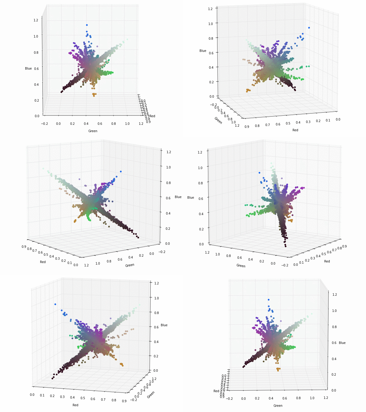
Very Deep CNN (19conv) first convolution filters 3D visualization

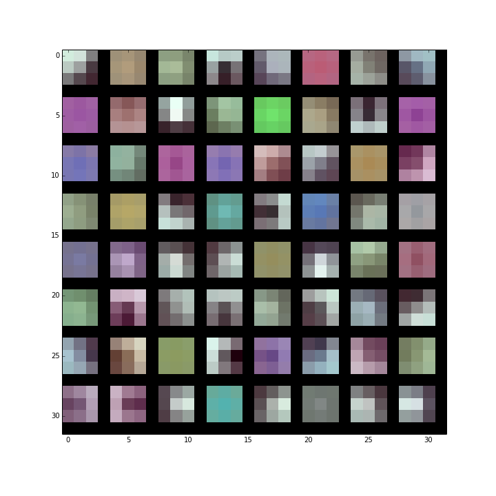
These are the filters of the first convolution layer of the very deep Convolutional Neural Network from Karen Simonyan and Andrew Zisserman available in the webpage www.robots.ox.ac.uk/~vgg/research/very_deep/ The authors have available an arXiv version of a paper in http://arxiv.org/abs/1409.1556

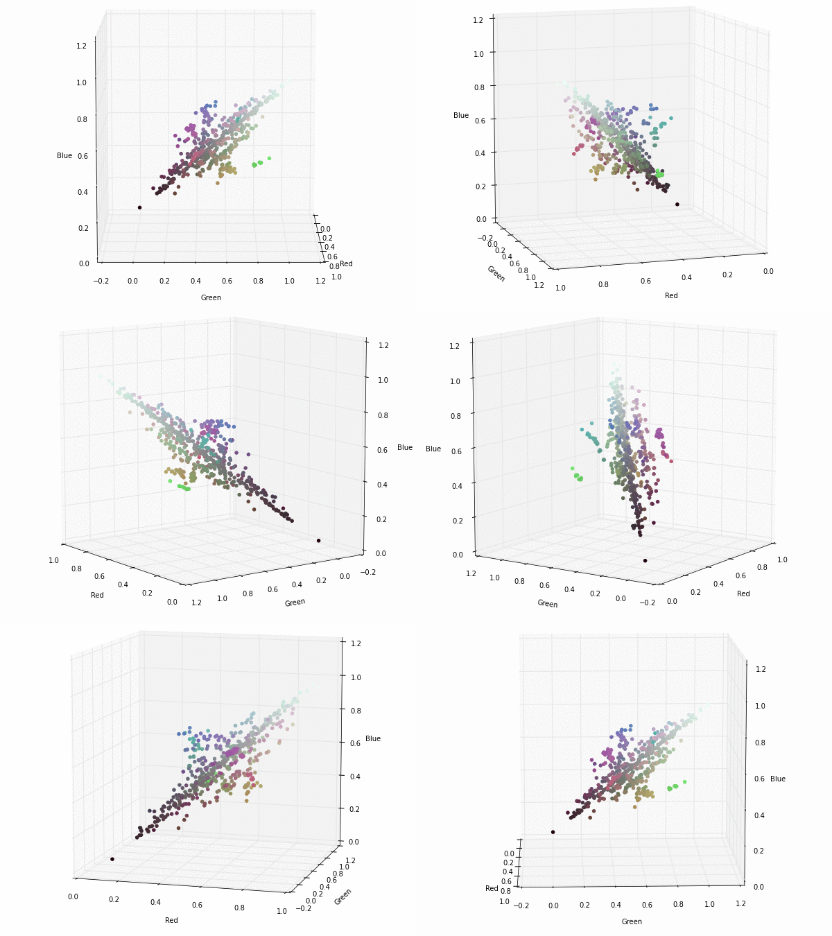
They got the 1st position for the localization task and the 2nd position in the classification task in ImageNet Challenge 2014. In order to get these results they evaluated different architectures with an increasing depth. This is the projection of the first convolutional layer filters in the RGB colorspace. Click on the images to see a 3D representation of the filters components.

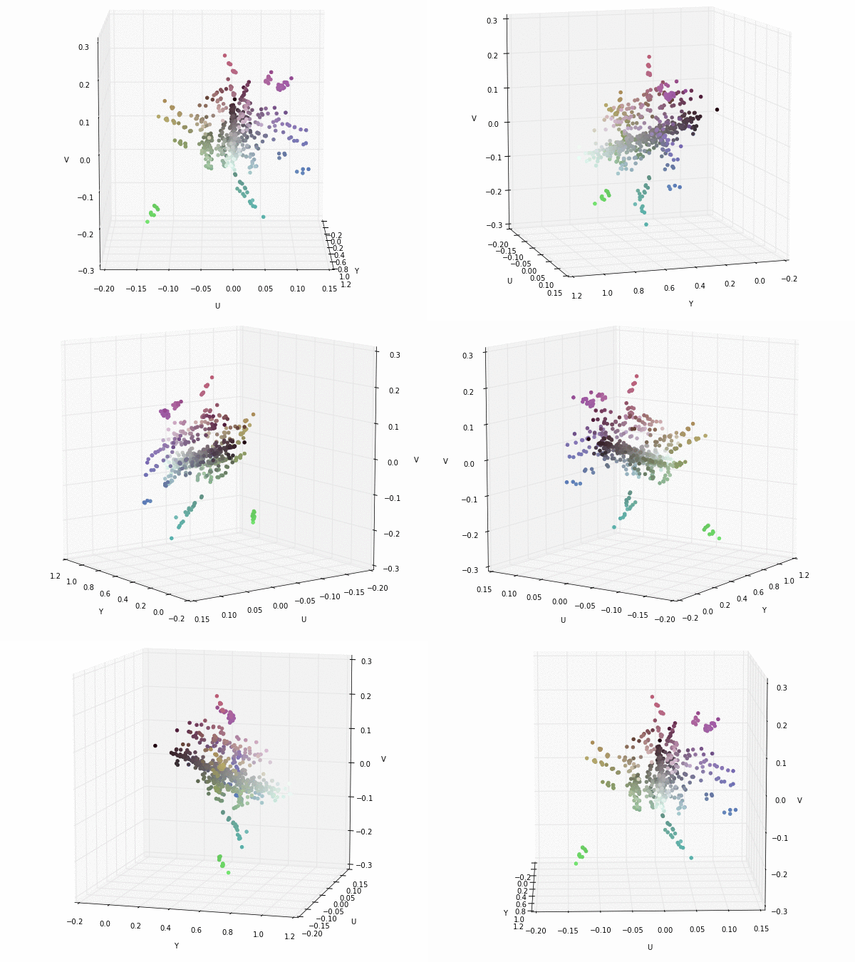
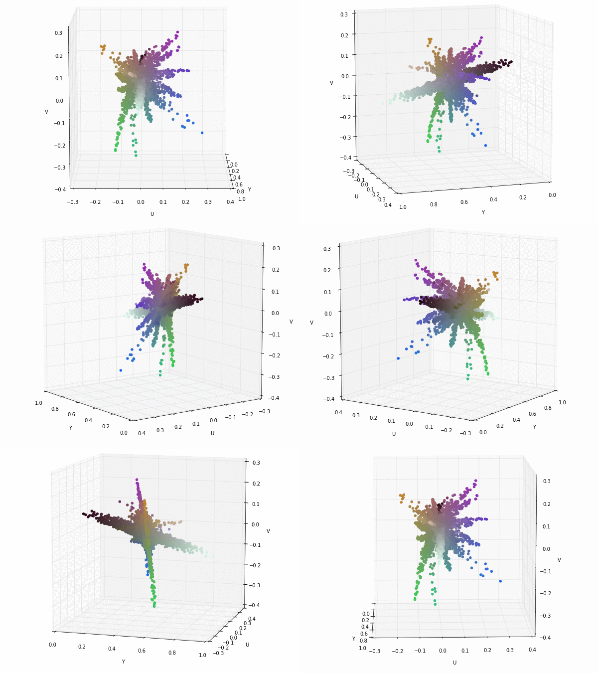
As in the Alexnet example we can do a linear transformation of the original RGB channels and visualize the same colors in the YUV colorspace. In this case the distribution of the points is not that clean and it seems that the distribution of the colours is more spread. This could be because the number of weights is very reduced 64x3x3x3 + 64 = 1792, compared to Alexnet 96x3x11x11 +96 = 34944.

If you find these interesting you can take a look at the results in my Master Thesis: webpage or the pdf and do not hesitate to ask me any question.

Alexnet first convolution filters 3D visualization

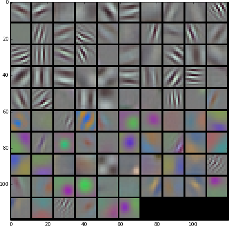
This are the filters of the first convolution layer of Alexnet network. If we look at them, they seem to be interested in luminance patterns (black-gray-white filters) and chrominance patterns (only the colour part without the black-gray-white component). This means that at the beginning the filters are specialized on this two typical situations and after that in the next convolution layer they could be appropriately merged.

To illustrate that, this is the projection of each pixel of the filters (they are really weight vectors with three components red-green-blue). Click on the images to see a 3D representation of the filters components.

If we apply a transformation to YUV colorspace; also known as YCbCr for digital images. We can see that the Y component (luminance) nearly gets their own axis while UV components (chrominance) are strongly correlated but slightly uncorrelated with the Y component. This means that they could be separated without any problem when training a CNN.

If you find these interesting you can take a look at the results in my Master Thesis: webpage or the pdf and do not hesitate to ask me any question.

Alexnet Graphviz visualization

Visualization of Alexnet using Graphviz. The example is a PNG as Blogger does not accept vectorial images like SVG or PDF. However, with the code below it is possible to generate a PDF calling the program "dot" with the next command:

dot -Tpdf alexnet.gv -o alexnet.pdf
# or an SVG
dot -Tsvg alexnet.gv -o alexnet.svg

alexnet.gv

// ================================================= //
// Author: Miquel Perello Nieto                      //
// Web:    www.perellonieto.com                      //
// Email:  miquel.perellonieto at aalto dot fi       //
// ================================================= //
//
// This is an example to create Alexnet Convolutional Neural Network
// using the opensource tool Graphviz.
//
// Tested with version:
//
//      2.36.0 (20140111.2315)
//
// To generate the graph as a PDF just run:
//
//      dot -Tpdf alexnet.gv -o alexnet.pdf
//
// One think to have in mind is that the order of the nodes definition modifies
// nodes position.

digraph Alexnet {
    // ================================== //
    //  GRAPH OPTIONS                     //
    // ================================== //

    // From Top to Bottom
    rankdir=TB;

    // Tittle possition: top
    labelloc="t";
    // Tittle
    label="Alexnet";

    // ================================== //
    //  NODE SHAPES                       //
    // ================================== //
    //
    // There is a shape and color description for each node
    // of the graph.
    //
    // It can be specified individually per node:
    //      first_node [shape=circle, color=blue];
    //
    // Or for a group of nodes if specified previously:
    //      node [shape=circle, color=blue];
    //      first_node;
    //      second_node;
    //

    // Data node
    // =========

    data [shape=box3d, color=black];

    // Label node
    // =========

    label [shape=tab, color=black];

    // Loss function node
    // ==================

    loss [shape=component, color=black];

    // Convolution nodes
    // =================
    //
    // All convolutions are a blue inverted trapezoid
    //

    node [shape=invtrapezium, fillcolor=lightblue, style=filled];
    conv1;
    conv3;
    // Splitted layer 2
    // ================
    //
    //  Layers with separated convolutions need to be in subgraphs
    //  This is because we want arrows from individual nodes but
    //  we want to consider all of them as a unique layer.
    //

    subgraph layer2 {
        // Convolution nodes
        //
        node [shape=invtrapezium, fillcolor=lightblue, style=filled];
        conv2_1;
        conv2_2;
        node [shape=Msquare, fillcolor=darkolivegreen2, style=filled];
        relu2_1;
        relu2_2;
    }

    // Splitted layer 4
    // ================
    //

    subgraph layer4 {
        // Convolution nodes
        //
        node [shape=invtrapezium, fillcolor=lightblue, style=filled];
        conv4_1;
        conv4_2;
        node [shape=Msquare, fillcolor=darkolivegreen2, style=filled];
        relu4_1;
        relu4_2;
    }

    // Splitted layer 5
    // ================
    //

    subgraph layer5 {
        // Convolution nodes
        //
        node [shape=invtrapezium, fillcolor=lightblue, style=filled];
        conv5_1;
        conv5_2;
        // Rectified Linear Unit nodes
        //
        node [shape=Msquare, fillcolor=darkolivegreen2, style=filled];
        relu5_1;
        relu5_2;
    }

    // Rectified Linear Unit nodes
    // ============================
    //
    // RELU nodes are green squares
    //

    node [shape=Msquare, fillcolor=darkolivegreen2, style=filled];
    relu1;
    relu3;
    relu6;
    relu7;

    // Pooling nodes
    // =============
    //
    // All pooling nodes are orange inverted triangles
    //

    node [shape=invtriangle, fillcolor=orange, style=filled];
    pool1;
    pool2;
    pool5;

    // Normalization nodes
    // ===================
    //
    // All normalization nodes are gray circles inside a bigger circle
    // (it reminds me a 3 dimmensional Gaussian looked from top)
    //

    node [shape=doublecircle, fillcolor=grey, style=filled];
    norm1;
    norm2;

    // Fully connected layers
    // ======================
    //
    // All fully connected layers are salmon circles
    //

    node [shape=circle, fillcolor=salmon, style=filled];
    fc6;
    fc7;
    fc8;

    // Drop Out nodes
    // ==============
    //
    // All DropOut nodes are purple octagons
    //

    node [shape=tripleoctagon, fillcolor=plum2, style=filled];
    drop6;
    drop7;

    // ================================== //
    //  ARROWS                            //
    // ================================== //
    //
    // There is a color and possible a label for each
    // arrow in the graph.
    // Also, some nodes has connections going in and
    // going out.
    //
    // The color can be specified individually per arrow:
    // first_node -> second_node [color=blue, style=bold,label="one to two"];
    //
    // Or for a group of nodes if specified previously:
    //  edge [color=blue];
    //  first_node -> second_node;
    //  second_node -> first_node;
    //  second_node -> third_node;
    //

    //
    // LAYER 1
    //

    data -> conv1 [color=lightblue, style=bold,label="out = 96, kernel = 11, stride = 4"];

    edge [color=darkolivegreen2];
    conv1 -> relu1;
    relu1 -> conv1;

    conv1 -> norm1 [color=grey, style=bold,label="local_size = 5, alpha = 0.0001, beta = 0.75"];
    norm1 -> pool1 [color=orange, style=bold,label="pool = MAX, kernel = 3, stride = 2"];

    pool1 -> conv2_1 [color=lightblue, style=bold,label="out = 256, kernel = 5, pad = 2"];
    pool1 -> conv2_2 [color=lightblue, style=bold];

    //
    // LAYER 2
    //

    edge [color=darkolivegreen2];
    conv2_1 -> relu2_1;
    conv2_2 -> relu2_2;
    relu2_1 -> conv2_1;
    relu2_2 -> conv2_2;

    conv2_1 -> norm2 [color=grey, style=bold,label="local_size = 5, alpha = 0.0001, beta = 0.75"];
    conv2_2 -> norm2 [color=grey, style=bold];
    norm2 -> pool2 [color=orange, style=bold,label="pool = MAX, kernel = 3, stride = 2"];

    pool2 -> conv3 [color=lightblue, style=bold,label="out = 384, kernel = 3, pad = 1"];

    //
    // LAYER 3
    //

    conv3 -> relu3 [color=darkolivegreen2];
    relu3 -> conv3 [color=darkolivegreen2];

    conv3 -> conv4_1 [color=lightblue, style=bold,label="out = 384, kernel = 3, pad = 1"];
    conv3 -> conv4_2 [color=lightblue, style=bold];

    //
    // LAYER 4
    //

    edge [color=darkolivegreen2];
    conv4_1 -> relu4_1;
    relu4_1 -> conv4_1;
    conv4_2 -> relu4_2;
    relu4_2 -> conv4_2;

    conv4_1 -> conv5_1 [color=lightblue, style=bold, label="out = 256, kernel = 3, pad = 1"];
    conv4_2 -> conv5_2 [color=lightblue, style=bold];

    //
    // LAYER 5
    //

    edge [color=darkolivegreen2];
    conv5_1 -> relu5_1;
    relu5_1 -> conv5_1;
    conv5_2 -> relu5_2;
    relu5_2 -> conv5_2;

    conv5_1 -> pool5 [color=orange, style=bold,label="pool = MAX, kernel = 3, stride = 2"];
    conv5_2 -> pool5 [color=orange, style=bold];

    pool5 -> fc6 [color=salmon, style=bold,label="out = 4096"];
    fc6 -> relu6 [color=darkolivegreen2];
    relu6 -> fc6 [color=darkolivegreen2];
    fc6 -> drop6 [color=plum2, style=bold,label="dropout_ratio = 0.5"];
    drop6 -> fc6 [color=plum2];

    //
    // LAYER 6
    //

    fc6 -> fc7 [color=salmon, style=bold,label="out = 4096"];

    //
    // LAYER 7
    //

    fc7 -> relu7 [color=darkolivegreen2];
    relu7 -> fc7 [color=darkolivegreen2];
    fc7 -> drop7 [color=plum2, style=bold,label="dropout_ratio = 0.5"];
    drop7 -> fc7 [color=plum2];

    fc7 -> fc8 [color=salmon, style=bold,label="out = 1000"];

    //
    // LAYER 8
    //

    edge [color=black]
    fc8 -> loss;
    label -> loss;
}

If you find these interesting you can take a look at the results in my Master Thesis: webpage or the pdf and do not hesitate to ask me any question.

Upper triangular matrix

Function to get the index of a matrix that is storing the upper triangular part of a square matrix.
I found this function in the bottom source, but I had to add the offset.

source: original function without offset

Function

In [1]:

def upper_triangular_index(n, r, c, k=0):
    """
    Returns the index of an array that is storing an
    upper triangular matrix. In this case the matrix
    has to be square and only accepts zero or possitive
    offsets.
    n = square matrix length
    r = actual row
    c = actual column
    k = diagonal possitive offset
    """
    return (n*r-k)+c-((r*(r+1))/2)-r*k

Some examples

In [2]:

import numpy as np

In [3]:

N = 3
keys = range(N)
matrix = np.ones((N,N), dtype=int)*-1

Small example without offset

In [4]:

offset=0
for key1 in keys:
    for key2 in keys:
        if key1+offset <= key2:
            matrix[key1,key2] = \
                upper_triangular_index(N, key1, 
                                       key2, k=offset)
print matrix

[[ 0  1  2]
 [-1  3  4]
 [-1 -1  5]]

Small example with offset = 1

In [5]:

matrix = np.ones((N,N), dtype=int)*-1
offset=1
for key1 in keys:
    for key2 in keys:
        if key1+offset <= key2:
            matrix[key1,key2] = \
                upper_triangular_index(N, key1, 
                                       key2, k=offset)
print matrix

[[-1  0  1]
 [-1 -1  2]
 [-1 -1 -1]]

Large example with offset = 3

In [6]:

N = 9
keys = range(N)
matrix = np.ones((N,N), dtype=int)*-1

In [7]:

offset=3
for key1 in keys:
    for key2 in keys:
        if key1+offset <= key2:
            matrix[key1,key2] = \
              upper_triangular_index(N, key1, 
                                     key2, k=offset)
print matrix

[[-1 -1 -1  0  1  2  3  4  5]
 [-1 -1 -1 -1  6  7  8  9 10]
 [-1 -1 -1 -1 -1 11 12 13 14]
 [-1 -1 -1 -1 -1 -1 15 16 17]
 [-1 -1 -1 -1 -1 -1 -1 18 19]
 [-1 -1 -1 -1 -1 -1 -1 -1 20]
 [-1 -1 -1 -1 -1 -1 -1 -1 -1]
 [-1 -1 -1 -1 -1 -1 -1 -1 -1]
 [-1 -1 -1 -1 -1 -1 -1 -1 -1]]

3D visualization of some colorspaces

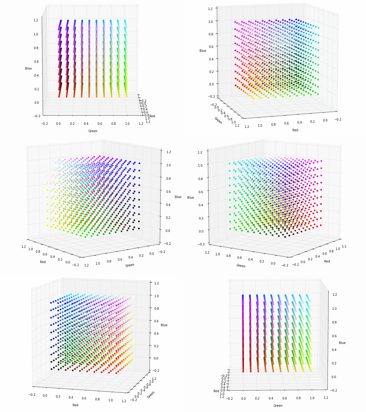
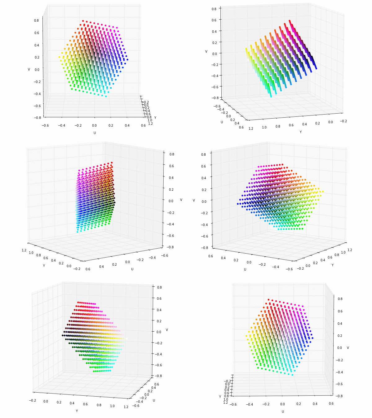
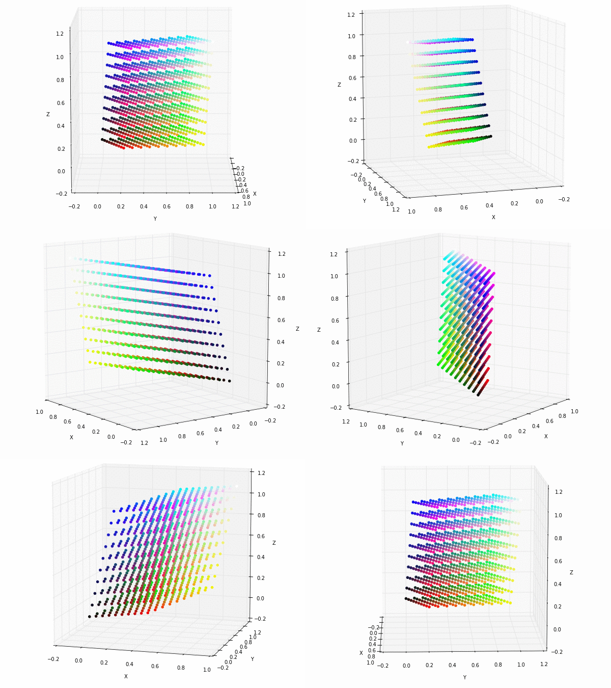
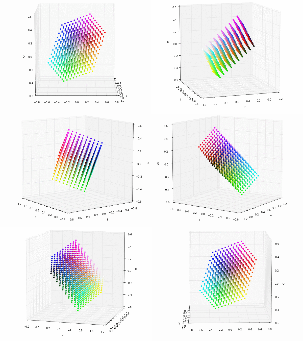
These are some GIF visualizations of an RGB cube in different colorspaces (Click in the images to see the 3D visualization, it can take some seconds to open as each visualization is about 11MB).

The original cube in the RGB colorspace:

RGB cube in the YUV colorspace:

RGB cube in the XYZ colorspace:

RGB cube in the YIQ colorspace:

If you find these interesting you can take a look at the results in my Master Thesis: webpage or the pdf and do not hesitate to ask me any question.

Perceptron training visualization

Visualization of a Perceptron trying to classify samples into two different categories.

 In this representation there is no bias involved,  the green arrow are the model weights and it defines an hyperplane orthogonal to them centred in the coordinates [0,0]. In each iteration the sample being tested is shown in orange. If the sample is in the wrong side of the hyperplane the vector representing the sample is shown, then the red vector is the same vector reescaled by the learning rate and it is summed to the weights vector. Then, the next sample is tested.